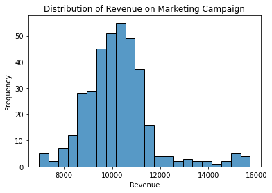
Summarizing Distributions for Marketers

Figure 1. Frequency Distribution of Revenue for a Marketing Campaign

You may have seen a plot that looks like this before. This plot is what is called a frequency distribution. In this case, it represents 365 days’ reported revenue, for an example marketing campaign.

You can glean many insights just by looking at this distribution. Currently, this data represents the number of times we saw a particular amount of revenue. We noticed that our campaign got us about $10,500 on 50 separate days. But what if we want to know how probable an outcome is? How do I answer the question, “What is the chance we make $10,500 tomorrow on this campaign?”

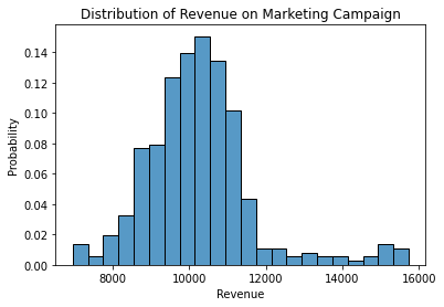
To answer that, we can quickly transform our data to look at probabilities by dividing our frequency counts by the number of times we observed the data. Since we’ve followed this campaign for a year (365 days), we can divide our frequencies by 365 to get our probabilities. You can see this visually since we know we had around 60 days to get $10,500 in revenue. The probability we reach $10,500 in income is 50/365 or about 14%.

Below is a visualization of all the different probabilities:

Figure 2. Probability Distribution of Revenue for a Marketing Campaign

There are some handy ways we can summarize different distributions. For example, if someone asks us, “How much revenue do you expect to get from this campaign?,” we may respond by saying, “On average, we get $10,267.23.”

When looking at marketing data, it is common to find outliers. In our example of campaign revenue, we frequently see outliers due to seasonality, promotions, or holidays. For example, we may not want our marketing efforts to get credit because of Black Friday.

You can see in Figure 2 above that some values look out of place between $13,000 and $16,000. Visually, you can see that the data is skewed, and because of this skew, we may want to look at the median of this distribution instead of the mean. In the example above, the median is $10,166.97. Which you choose is up to you. I recommend looking at the median when the data is severely skewed. That said, considering both is always helpful.

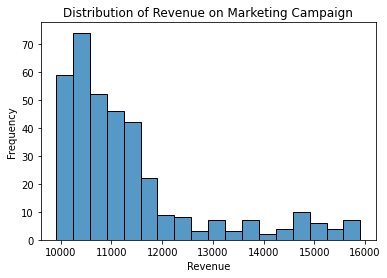
Figure 3 below shows an example where considering both the mean and median is useful:

Figure 3. Frequency Distribution of Marketing Revenue with Skew

Figure 3 shows that the mean is $11,348.84, and the median is $10,893.89. Significant anomalies can skew the results even more. This distribution is considered right-skewed; the outliers are on the right. The inverse is called a left-skewed distribution, where the outliers are on the left.

The mean is always on the side of where the outliers are, and the median is always to the left of the mean. It’s helpful to remember the median as being more robust to outliers. Therefore, the median is always farther away from the outliers when compared to the mean.

Imagine that we want to compare two different marketing campaigns. Both of these campaigns have consistent spending per day for an entire year. Say, we spend, on average, $10,000 a day on Campaign One and $5,000 a day on Campaign Two. Now, we want to measure the performance of these campaigns to decide which campaign we want to invest more money into.

Comparison of Two Marketing Campaigns and their Revenue

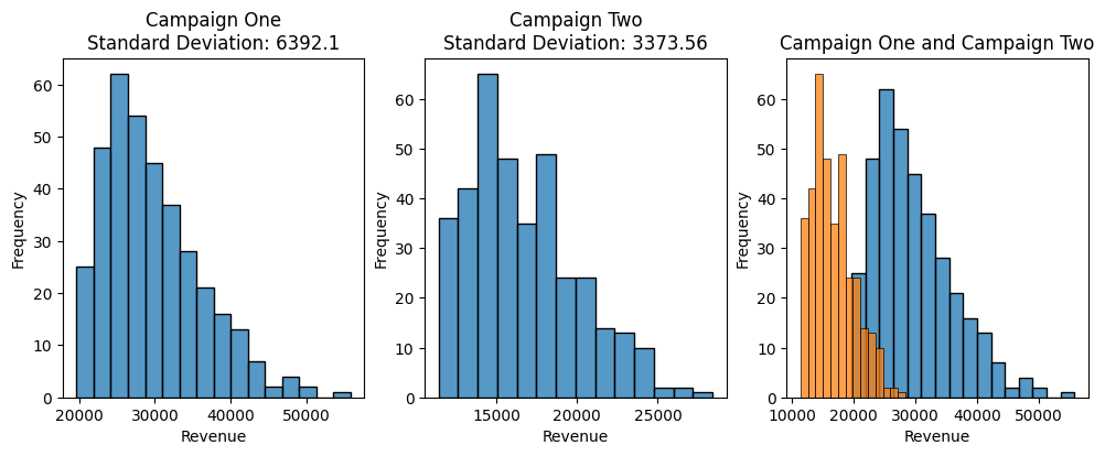
Above, we can see that Campaign One has a higher maximum return than Campaign Two. Campaign One’s mean is around $29,603.26, while Campaign Two’s mean is around $16,652.23. Again, this means that, on average, Campaign One gets us ~$29k a day, and Campaign Two gets us ~$16k a day.

Considering our average return, we may choose Campaign One over Campaign Two, which is okay, but what if we want to be confident in the returns of our campaigns? In this case, we need to ask, “How certain are we that Campaign One will return $29k on any given day versus how certain are we that Campaign Two will return $16k on any given day?”

When answering questions about our expectations, the standard deviation is crucial to include. The standard deviation is a metric that helps us quantify the dispersion of the data. The higher the standard deviation, the more dispersed the data is. Like the mean and median, the standard deviation is in the same units as the data.

Visually, if you look at the plot on the far right, you can see that the orange data is much closer together than the blue data. Numerically, you can see that the standard deviation for campaign one is much higher (double) than campaign two, $6,392 and $3,373, respectively. Again, this means that we have more conviction that spending on Campaign Two will yield consistent results versus Campaign One because there is less variation in the daily data.

We frequently want to look at the standard deviation in combination with the mean. So, Campaign One has a mean of $29,603.26 +/- $6,392 and Campaign Two has a mean of $16,652.23 +/- $3,373. We read this as “Campaign One has a mean of $29,603.26 plus or minus $6,392.”

A good rule of thumb is that it’s an outlier if data exceeds two standard deviations above the mean. So, for Campaign One, if we saw a data point ($29,603.26 + $12,784), it’s an outlier. As I’ve stated, standard deviations are primarily used to describe data spread, however, reliability of expectations are better framed in terms of confidence intervals or statistical hypothesis testing.

Another metric you may hear about is called the variance. Variance tells us if our data is close together (low variance) or spread apart (high variance). It helps us understand how much the data points “vary” from the average.

This definition makes the standard deviation sound very similar to the variance, and there is a good reason for this: To calculate the standard deviation, we calculate the variance first. Variance is the squared version of the standard deviation. This square unit measurement is because variance involves squaring the differences between individual data points and the mean. It’s a way to quantify the spread of data, and squaring the differences ensures that negative and positive differences don’t cancel each other out, which would be the case if you summed the differences without squaring them.

For data analysis, the standard deviation is usually preferred over the variance because the standard deviation is easier to interpret. After all, it is in the same units as the mean.

Key Points:

To convert raw counts (frequencies) into probabilities you can divide each frequency by the total count (or sum of frequencies).
You should use the mean, median, and standard deviation when summarizing any distribution of data.
The median is more robust to outliers than the mean.
A distribution’s skew is determined by where the outliers are. A left-skewed distribution has outliers on the left side. A right-skewed distribution has outliers on the right side.
Standard deviations are useful for discussing how spread out data is.

Now that we’ve seen why the mean, median, standard deviation and variance are useful for analysis, it’s prudent to discuss how we calculate them. Warning, there will be some mathematical notation in this section so skip it if you want but I’ll include it for the curious reader.

For all examples I am using an array: [1, 2, 3, 4, 5]

1. Mean (Average):

$\text{Mean} (\mu) = \frac{1}{n} \sum_{i=1}^{n} x_i$

Add up all the numbers in the list.
Divide the sum by the total number of values in the list.

Example:

Sum = 1 + 2 + 3 + 4 + 5 = 15
Total number of values = 5
Mean = Sum / Total number of values = 15 / 5 = 3

Python Example:

import numpy as np
vals = np.array([1, 2, 3, 4, 5])
np.mean(vals)

2. Median:

Arrange the numbers in the list in ascending order.
If the total number of values is odd, the median is the middle value.
If the total number of values is even, the median is the average of the two middle values.

Example:

Arranged list in ascending order: [1, 2, 3, 4, 5]
Since the total number of values is odd, the median is the middle value, which is 3.

Python Example:

import numpy as np
vals = np.array([1, 2, 3, 4, 5])
np.median(vals)

3. Variance:

$\text{Variance} (\sigma^2) = \frac{1}{n} \sum_{i=1}^{n} (x_i - \mu)^2$

Calculate the mean (average) of the numbers.
For each number in the list, subtract the mean, square the result, and sum all the squared differences.
Divide the sum of squared differences by the total number of values minus 1 (this is called “degrees of freedom”).

Example:

Mean (calculated earlier) = 3
Calculate squared differences:
- (1 – 3)^2 = 4
- (2 – 3)^2 = 1
- (3 – 3)^2 = 0
- (4 – 3)^2 = 1
- (5 – 3)^2 = 4
Sum of squared differences = 10
Degrees of freedom = 5 – 1 = 4
Variance = Sum of squared differences / Degrees of freedom = 10 / 4 = 2.5

Python Example:

import numpy as np
vals = np.array([1, 2, 3, 4, 5])
np.var(vals)

4. Standard Deviation:

$\text{Standard Deviation} (\sigma) = \sqrt{\text{Variance}}$

Take the square root of the variance.

Example:

Variance (calculated earlier) = 2.5
Standard Deviation = √Variance = √2.5 ≈ 1.58

So, for the list of numbers [1, 2, 3, 4, 5]:

Mean: 3
Median: 3
Variance: 2.5
Standard Deviation: Approximately 1.58

Python Example:

import numpy as np
vals = np.array([1, 2, 3, 4, 5])
np.std(vals)