Understanding Adstock Effects in Media Mix Modeling

As we know, marketing impacts are not always simple, discrete events. Marketing dollars spent today impact revenue tomorrow. If we ignore the impact of marketing efforts over time, we could be undervaluing our efforts. One way to capture the impact of marketing over time is through Adstock effects. Adstock functions aim to capture the prolonged influence of advertising beyond its immediate deployment. Utilizing Adstock functions is crucial for analysts assessing marketing effectiveness and optimizing future spending.

A Brief History of Adstock Effects

Simon Broadbent coined the term Adstock in the 1970s as part of his work measuring the effectiveness of TV ads. The term refers to inventory stock, where the impact of advertising accumulates and then gradually depletes over time. Measuring marketing through Adstock allows us to estimate the lasting impact of marketing campaigns, shifting the focus from immediate outcomes to longer-term effects.

Methodologies for Measuring Adstock

When selecting an Adstock function, we have no shortage of choices. The concept for all Adstock is essentially the same: we have some peak exposure value, which then decays over time. We get more parameters to estimate as the complexity we want our functions to model increases. This means we must select a model that matches our intuition and makes sense given our data. As a rule of thumb, the more parameters we estimate, the more data to which we want access. In the following section, I’ll provide three different Adstock functions, which range in complexity and flexibility.

Simple Adstock Model

The simple Adstock model applies a single decay rate to past advertising expenditures to model their lingering effect. One of the assumptions of this model is that the impact of advertising peaks at the same time as the spend. We can represent the function as follows:

$A_t = X_t + \theta_tA_{t-1}$

where:

$A_t$ is the Adstocked value of advertising spend at time $t$
$X_t$ is the advertising spend at time $t$
$\theta$ is the decay rate $0 < \theta < 1$
$A_{t-1}$ is the Adstocked value from the previous period

Figure 1. Simple Adstock Function with Different Values for Theta

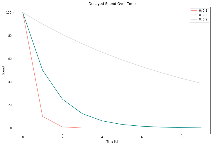
As you can see from Figure 1, with this Adstock function, we only get one shape, which can have different decay rates. We can control our decay rate based on our $\theta$ parameter.

In this function, we only have one parameter to estimate: $\theta$ . In this case, $\theta$ controls the decay we witness in a marketing effort. In this simple function, $\theta$ is constant and does not vary over time.

The Pros and Cons

This simple function is helpful as a starting point because it’s easy to understand and explain to our downstream users. It’s also easy to implement in multiple frameworks and provides a solid baseline to which we can compare more complicated functions.

Simplicity can come with downsides, though. In this function, we assume a uniform decay wherever the function is employed, which means we could ignore channel or campaign diversity. This function also ignores time, so we consider that our decay is static across time, which may cause an issue when fitting and using our function to forecast.

We may fit the function separately per campaign or channel to overcome some of these shortcomings. Fitting multiple functions adds more complexity and training time but would allow us to learn different decay rates depending on the input. We can also transform the data before putting it through our function by taking a rolling average of the input value. Transforming the data this way would allow us to measure changing market conditions.

Variable Adstock Model

The variable Adstock model introduces different decay rates for lags, acknowledging that the impact of advertising may vary over time. This model can be represented as:

$A_t = \sum_{i=0}^{n} \theta_i \times X_{t-i}$

where:

$A_t$ is the Adstocked value of advertising spend at time $t$
$X_{t-i}$ is the advertising spend at time $t-1$
$\theta_i$ is the decay rate $0 < \theta < 1$ at period $i$

As you can see, this function introduces two new symbols: the summation symbol ( $\sum$ ) and the $i$ subscript. In this function, we have $i$ $\theta$ s. Each $\theta_i$ represents the decay rate for the advertising spend $i$ periods ago. We must sum each decayed spend for each period $i$ . We denote each period’s decayed spend by $\theta_i \times X_{t-i}$ .

variable adstock model — Figure 2: Variable Adstock Model With Different Values for Theta

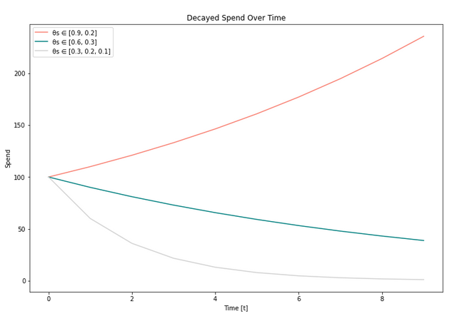
In Figure 2, you can see how this function now represents even more shapes of Adstock. Notice how we can now have a compounding effect of spending the closer $\theta$ is to 1. In other words, spending two days ago impacts today, spending yesterday impacts today, and today’s expenditures impact today. In summation (pun intended), the revenue I get today is also a function of my spending $i$ days ago.

The Pros and Cons

The variable Adstock model accounts for changing market conditions through different decay rates at various time lags. Inserting time into this equation gives us a more nuanced view of how our marketing efforts impact saturation and decay, leading to improved model precision.

With the increased number of parameters, the variable Adstock model generalizes more complicated shapes than the traditional Adstock model, and the relative downsides are limited. Since introducing more model parameters, we further complicate model fitting, and the increased complexity necessitates more data and compute time.

Dynamic Adstock Model

Dynamic Adstock models incorporate time-varying decay rates that can adjust based on external factors or internal performance metrics. This approach can be conceptualized as:

$A_t = f(\cdot) \times X_t + ( 1- f(\cdot) \times A_{t-1})$

where

$A_t$ is the Adstocked value of advertising spend at time $t$
$X_t$ is the advertising spend at time $t$
$f(\cdot)$ is a function which approximates decay rates based on inputs
$A_{t-1}$ is the Adstocked value from the previous period

Due to the inclusion of a generic $f(\cdot)$ function, this version of Adstock is much more flexible than the others. However, the analyst determines an appropriate function, and specifying this function is far from straightforward.

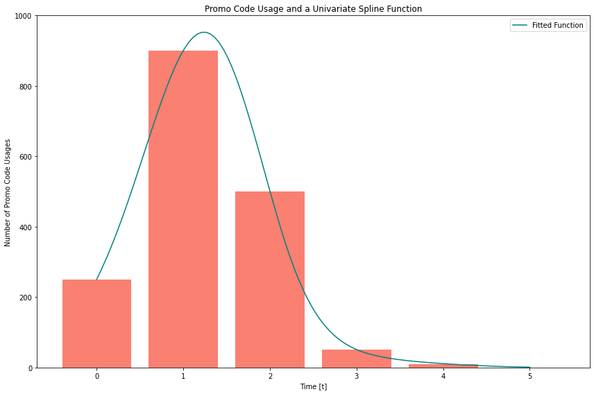
An appropriate time to use this model maybe when we have some existing data that suggests how our marketing decays over time—for example, influencer marketing for an e-commerce company. In influencer marketing, it is not uncommon for influencers to use promotion codes to get a revenue share of the product. Analysts can access which orders have a promo code attached to them. Using this data, we can learn a function that models the decay of this usage and use it to estimate how our Adstock decays over time.

Figure 3: Estimated $f(\cdot)$ Using Promo Code Usage Over Time

Figure 3: Estimated $f(\cdot)$ Using Promo Code Usage Over Time

In Figure 3, you can see the counts of the promo code usage and a function that fits the shape. In this example, the function is a proxy for the number of impressions an influencer had, which provides a shape for how the influencer’s impact decays over time. This forms an intuitive function for estimating Adstock.

The Pros and Cons

The most significant benefit of using the Dynamic Adstock model is its flexibility. The analyst can select whichever function they believe best models our decay rates. As I’ve said, this can be incredibly powerful, especially when decay is latent, but we have data that we can use as a proxy. Another benefit of this type of model is the general paradigm. We can select any function we believe appropriately models $A_t$ and any function we want for $f(\cdot)$ .

Again, the analyst selects the function $f(\cdot)$ , and employing the wrong function can lead to poor estimation of the Adstock function itself and the overarching MMM. Depending on the type of function selected, overfitting may become a problem, leading to biased and unreliable results. Also, depending on the complexity of the model, we may increase the amount of data needed and the computation required to estimate the function.

Conclusion

Measuring Adstock effects is an intricate but crucial component of Media Mix Modeling, enabling marketers to capture the total value of their advertising spend over time. From the simple Adstock model’s straightforward simplicity to the variable Adstock model’s nuanced flexibility, and the adaptability of the dynamic Adstock model, each approach offers unique benefits and faces specific challenges. By carefully selecting and tailoring the Adstock measurement methodology to their particular needs, marketers can enhance their understanding of advertising effectiveness, leading to more informed decision-making and optimized marketing strategies.

1) Broadbent, S. (1979) “One Way TV Advertisements Work”, Journal of the Market Research Society Vol. 23 no.3