Utilizing Trend Terms in Media Mix Modeling

Trend Terms in Modern Marketing Mix Modeling

Accurately measuring and predicting trends is paramount for success in the ever-evolving marketing landscape. Marketing Mix Modeling (MMM) has emerged as a powerful tool, enabling marketers to dissect the impact of various marketing activities on sales and other key performance indicators. Within MMM, incorporating trend terms plays a crucial role in capturing and understanding the underlying patterns in data. In this article, we delve into three essential trend terms: linear trend, linear trend with change points, and local linear trend, exploring their significance and applications in modern marketing analytics.

Linear Trend

At its core, a linear trend is a straightforward representation of data points linearly evolving. It assumes a consistent rate of change over the entire duration of the analyzed period. In MMM, incorporating a linear trend term allows marketers to capture the overall growth or decline in sales that occurs steadily over time, irrespective of other factors.

Consider a scenario where a company experiences a gradual increase in sales over several years due to market expansion or improved brand recognition. Analysts can accurately quantify this long-term growth trend by including a linear trend term in the model. This insight is invaluable for strategic decision-making, such as setting realistic sales targets or assessing the effectiveness of marketing campaigns against the backdrop of organic growth.

Mathematically, the linear trend is straightforward and can be expressed as a simple linear regression model:

$y_t = \beta_0 + \beta_1 t + \epsilon_t$

where:

$y_t$ represents the observed value of the dependent variable at time $t$
$\beta_0$ is the intercept coefficients
$\beta_1$ is the slope coefficient
$t$ denotes time as an independent variable
$\epsilon_t$ represents the error term at time $t$

In the above formulation $\beta_0$ represents are initial level, or the amount of revenue we have at $t = 0$ and $\beta_1$ represents the slope of the trend.

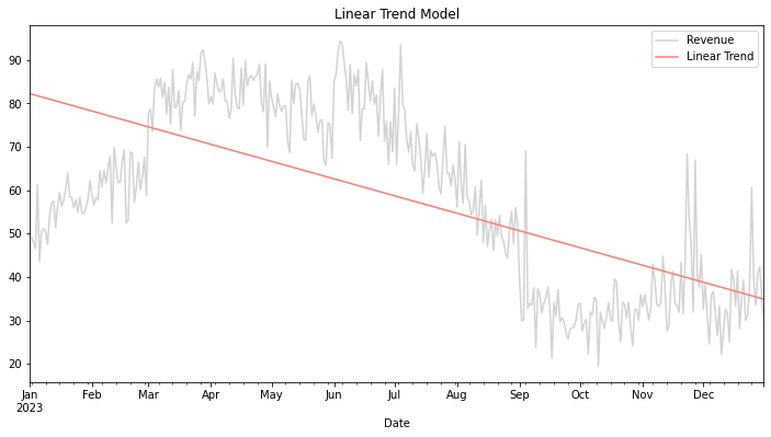
Linear trends have several upsides, making them a useful heuristic for modeling trends. Namely, they are simple. Everyone understands what a line looks like, and they are easy to communicate. On top of that, they offer a high degree of interpretability. The coefficient of a linear trend represents the initial starting point (the intercept) and the rate of change we expect to see over time. Lastly, If they are used in the proper context when we see a linear trend, they are very stable.

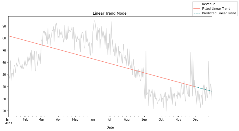
The downsides of linear trends stem from their limited flexibility. They have assumptions around linearity and a constant rate of change over time, making them poor choices in volatile environments or environments where we see a lot of outliers. You can see an example of this in Figure 1 where the trend poorly fits. Here you can see how taking a simplistic view of the underlying patterns in the data causes a high degree of overgeneralization.

Linear Trend with Change Points

While linear trends offer a simplified view of data progression, real-world scenarios often exhibit more complex dynamics characterized by abrupt shifts or changes in underlying patterns. Linear trend models with change points address this limitation by allowing for discontinuities in the trend line, signifying significant transitions in the market environment.

Imagine a company that experiences a sudden surge in sales following the launch of a new product line or implementing a disruptive marketing campaign. Traditional linear trend models struggle to capture such events’ immediate impact accurately. However, by incorporating change points into the analysis, marketers can pinpoint the precise moments when shifts in sales trajectory occur, enabling them to attribute changes to specific interventions or external factors.

These models are a nice extension of our standard linear trend model. The change points introduce discontinuities in the trend line to account for shifts in the trend. We can show this mathematically as follows:

$y_t = \beta_{0i} + \beta_{1i} t + \epsilon_t$

where:

$y_t$ represents the observed value of the dependent variable at time $t$
$i$ represents the index for each line segment
$\beta_0i$ are the intercept coefficients for each line segment
$\beta_1i$ are the slope coefficients for each line segment
$t$ denotes time as an independent variable
$\epsilon_t$ represents the error term at time $t$

Figure 2. Piecewise Linear Trend with Changepoints

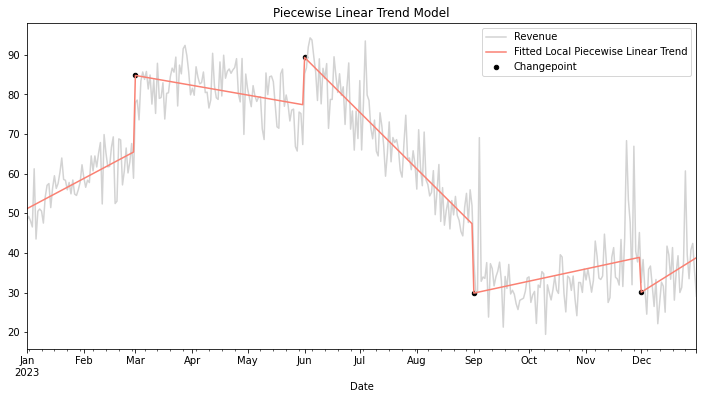
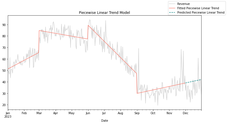
We can see in Figure 2 how we have specified 4 changepoints. This means that we get 5 line segments. As I generated the synthetic data for this myself, identification of the location of change points was easy but this isn’t always the case.

Adjusting the standard linear trend with change points allows an analyst to adjust for shifts or transitions in the trend behavior. If a business has clear areas where changes are detected, we can leverage this to provide granular insights into the magnitude of interventions or external factors influencing sales trajectories. Since we can capture discontinuities with change points and get different slopes for different segments, we have more flexibility for forecasting, which also improves our accuracy compared to standard linear trends.

As with most things, we increase the complexity as we increase the flexibility. Identifying change points requires a lot of familiarity with the business and its history. As such, we inject subjective judgment or arbitrary thresholds, introducing uncertainty into the modeling process and affecting the robustness of results. Linear trends with change points require larger datasets to detect meaningful shifts reliably, limiting their applicability in contexts where data availability is limited.

Local Linear Trend

While long-term trends provide valuable insights into overall market dynamics, they often mask short-term fluctuations or seasonality inherent in the data. Local linear trend models address this issue by introducing flexibility into trend estimation, allowing for capturing short-term variations while preserving the underlying trajectory.

In industries characterized by seasonal demand patterns, such as retail or tourism, local linear trend models capture the cyclicality of sales without conflating it with long-term growth trends. By distinguishing between short-term fluctuations and enduring trends, marketers can devise targeted strategies to capitalize on seasonal peaks or mitigate downturns effectively.

The local linear trend model is a time series model that allows the series’ level and slope to evolve over time, making it suitable for forecasting and analyzing time series with non-constant trends. We can show this model mathematically through three separate equations as follows:

$y_t = \mu_t + \epsilon_t$ [1]

$\mu_t+1 = \mu_t + \beta_t + \eta_{\mu, t}$ [2]

$\beta_t+1 = \beta_t + \eta_{\beta, t}$ [3]

where:

Equation 1 is the equation for the observations
Equation 2 is the equation for intercepts
Equation 3 is the equation for the slopes

and

$\mu_t$ is the intercept of the time series at time $t$
$\beta_t$ represents the slope of the time series at time $t$
$\eta_{\mu, t}$ represents the error (disturbance) to the intercept at time $t$
$\eta_{\beta, t}$ represents the error (disturbance) to the slope at time $t$

In those formulations, $\mu_t$ sets the current position of the series, and $\beta_t$ indicates the direction and magnitude of its immediate movement. The $\eta$ terms introduce stochastic elements to the intercept and slope of the time series, which is the reason for the local linear model’s flexibility. When we combine all of these elements, we allow the model to capture a wide range of time series behaviors, especially when the time series is subject to random shocks or when the underlying process is subject to change over time.

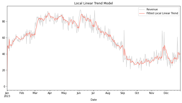
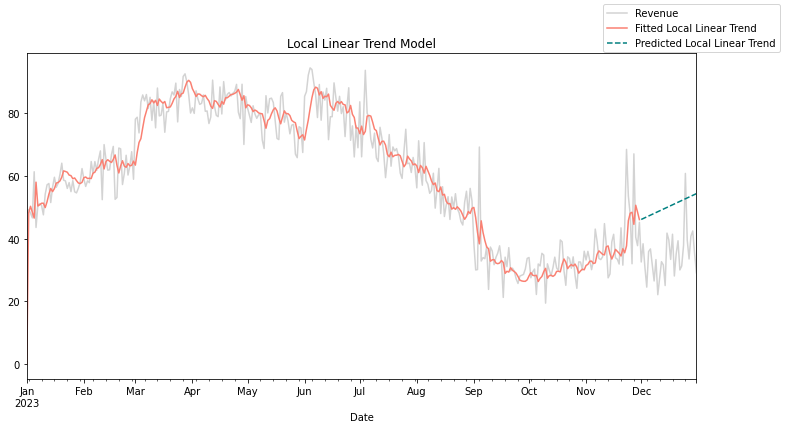
As can be seen in Figure 3, local linear trend models are adept at handling data with irregularities or outliers, offering robustness against noise or anomalies that may distort traditional trend analyses. This resilience enhances the reliability of MMM outputs, empowering marketers with actionable insights grounded in robust statistical methodologies.

While linear trends are good at estimating long-term movement, local linear trends offer flexibility in trend estimation by adapting to short-term fluctuations and preserving the underlying trajectory. This makes them incredibly useful and well-suited for capturing dynamic market behaviors. Local linear trends are more robust against outliers or irregularities in the data, enhancing the reliability of model outputs in noisy environments. These models provide granular insights into long-term trends and short-term variations, enabling marketers to differentiate between cyclical patterns and enduring growth trajectories effectively.

Local linear trends are much more complicated than linear-based trends, and implementing local linear trends requires a deep understanding of state space modeling and time series analysis techniques. Local linear trends also have more parameters, and selecting appropriate parameters for weighting functions or smoothing parameters requires careful calibration to achieve optimal model performance. These trend terms are also prone to overfitting, which may cause accuracy issues during forecasting. Interpreting local linear trends is not nearly as intuitive as interpreting traditional ones, as they involve dynamic interactions between trend components and random fluctuations over time.

Out of Sample Trend Forecasting

When looking at different trend terms, we care most about how well the trend captures the underlying patterns in the seen data and how well the model generalizes out-of-sample (on unseen data). All three trend functions above have different strengths, weaknesses, and abilities to generalize.

It is essential to understand that the information that the trend functions learn during training is all they have to use during inference. What I mean by this is that if the trend terms “see” a downward trend (the coefficients of the slopes are negative), it will assume that the unseen values are also trending downwards. Trend terms are only part of the picture, so we must never look at trend terms alone and pay special attention to models that allocate a high amount of the signal to the trend.

An example of this poor usage of trend terms was seen at Zillow when their usage of Facebook’s Prophet library caused an $8 billion drop in market cap, a $304 million operating loss, and 2,000+ jobs lost. This debacle isn’t Prophet’s fault. When property values increase for a while, these trend-oriented models will learn this upward momentum and use that in the trend for inference. The result? When property values are up and to the right, your forecasts are also up and to the right…which is fine until it’s not.

When building MMMs, we must take extra care to analyze the trend terms and see how they backtest across multiple swaths of data. When backtesting, we want to look back in time far enough to capture variability in the time series. To capture this variability, we must look back far enough to witness holidays, differing market conditions, and seasonality to ensure our model performs well across these conditions. Commonly, you’ll hear people recommend “at least two years of data.” This recommendation comes from the concept of capturing these effects.

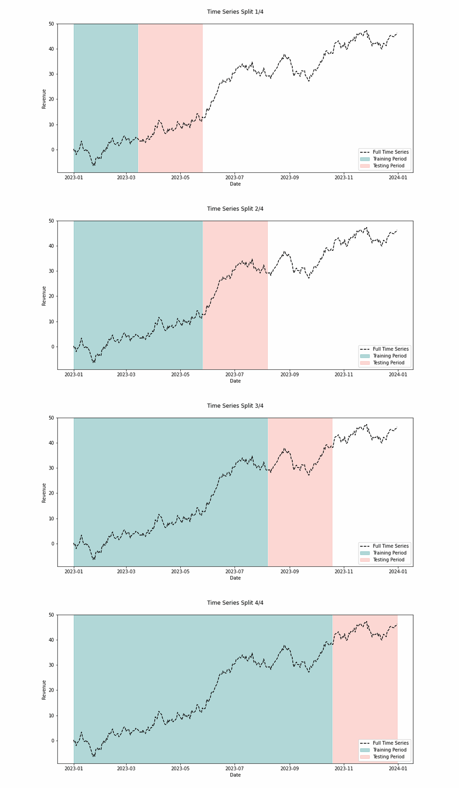
Figure 4. Visual Representation of Backtesting

In Figure 4, we can see how we approach backtesting. We need to train on different periods and conduct multiple forecasts measuring the error at each split. This way, we can honestly see how well our models can predict the future.

Figures 5-7 below show the results of a simple one-step backtest for the three trends we discussed above. As you can see, the in-sample fit does not always indicate the out-of-sample fit.

Figure 5. Backtest for Linear Trend Model

Figure 6. Backtest for Piecewise Linear Trend Model

Figure 7. Backtest for Local Linear Trend Model

Conclusion

In modern marketing analytics, effectively utilizing trend terms within MMM frameworks is essential for unlocking actionable insights and driving informed decision-making. Whether capturing long-term growth trajectories, adapting to sudden shifts in market dynamics, or navigating short-term fluctuations, trend terms offer a nuanced understanding of data patterns indispensable for marketers.

By embracing linear trends, linear trends with change points, and local linear trend models, marketers can gain a holistic view of their market performance, identify opportunities for optimization, and stay ahead of the curve in an increasingly competitive landscape. As the marketing landscape continues to evolve, leveraging the power of trend terms in MMM will remain a cornerstone of strategic decision-making, enabling companies to thrive in dynamic and unpredictable environments.

All code can be for here.