The Role of Linear Regression in Media Mix Modeling

To better navigate the intricacies of Media Mix Modeling (MMMs), it’s crucial to understand the foundational principles of regression models. The utility of regression models in media measurement has stood the test of time, serving as the bedrock for more sophisticated analytical approaches. Regression models have been a longstanding and integral tool in marketing. This article seeks to help the reader better understand regression models in the context of Media Mix Modeling.

Notation

To understand how we can use regression in media measurement, we must fully grasp related nomenclature and notation:

Independent Variables: Independent variables are the things that can vary in an experiment. For example, if you’re testing how a singular campaign impacts your total revenue, the amount of marketing spend (which you control) is the independent variable. It’s the “cause” you’re testing. Note that regression does not inherently imply causality.
- Notation: $X$ where $X$ could be a single variable or a feature matrix of multiple independent variables otherwise notated as $(X_1, X_2, ..., X_p)$
Dependent Variable: A dependent variable is what you’re trying to determine or measure in an experiment. It’s like the “effect.” Using the marketing example, the amount of store revenue would be the dependent variable because it’s dependent on how much you spend.
- Notation: $Y$
Coefficient: Coefficients are helper numbers that tell how much one thing influences another. In our marketing example, we’re figuring out how much revenue you get based on your marketing spend. The coefficient helps you understand how much your revenue changes for each extra dollar you spend.
- Notation: $\beta$ where $\beta$ could represent a single coefficient or a matrix of coefficients otherwise notated by $(\beta_1, \beta_2, ..., \beta_p)$
Intercept: The intercept represents the value of the dependent variable when the independent variable(s) are zero. In our marketing example, this translates to the revenue generated when we spend no money marketing.
- Notation: $\beta_0$
Error: Incorporating the error term in the regression formulation is essential because it signifies the unobserved influences on the dependent variable that the model cannot consider. This term captures the differences between the predicted and actual values, illustrating the inherent randomness or unexplained aspects in real-world data. In a practical scenario, such as our marketing example, inadvertently omitting a marketing channel or channels may manifest in the error term.
- Notation: $\epsilon$
Regression: Regression is a method that helps us understand the relationship between independent variables and a dependent variable. It provides a coefficient(s) that indicates the strength and direction of each factor’s influence on the outcome. Regression models are tools that analyze and quantify connections within data.
- Notation: $Y = \beta_0 + \beta_1 X_1 + \beta_2 X_2 + \ldots + \beta_p X_p + \epsilon$

The Linearity Assumption

One of the critical assumptions in linear regression (for media mix modeling) is that a linear relationship exists between marketing spend and revenue. However, we must recognize that the true relationship between advertising spending and revenue may sometimes be more complex (i.e., non-linear). Beginning with a simple linear model and then exploring more complex relationships based on the characteristics of the data is a decent starting point.

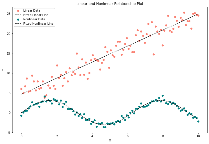
Figure 1. Linear Data Compared to Nonlinear Data

In Figure 1, the distinction between linear and nonlinear data is evident. Linear data looks like a line, while nonlinear data does not. While it is possible to fit a linear model to nonlinear data, it is imperative to recognize that this approach may yield a model that inadequately represents the underlying dynamics. Such misrepresentation can significantly influence decision-making based on the model’s inferences. In constructing MMMs, it is crucial to prioritize understanding the data’s shape and align model assumptions accordingly. The fidelity of the model’s reflection of data dynamics is pivotal in ensuring robust and reliable insights.

Synthetic Data Generation

We are about to build our first MMM, but it’s vital to understand synthetic data before we begin. We artificially generate data that mimics the patterns and characteristics of real-world data. This data is then called synthetic. In media mix modeling, we use synthetic data to validate our models by offering a controlled environment for testing and assessment.

This artificially generated data allows us to play the role of god because we get to control the dataset’s characteristics precisely. Synthetic data is precious in media mix model validation because it enables the creation of scenarios with known relationships between variables.

We craft datasets that mirror real-world data’s expected patterns and complexities, allowing us to assess how well our models capture the underlying dynamics. As researchers and users of MMMs, we must understand these patterns and the limitations our models have to describe them.

Linear models assume a straight-line relationship between the independent and dependent variables. Due to this linearity assumption, we must create our synthetic data with linear relationships; otherwise, we get a suboptimal representation of the underlying relationships, potentially resulting in poor model performance and inaccurate predictions.

To start, we can create 365 days’ worth of data. We do this by sampling randomly from the uniform distribution 365 times. This sampling will generate 365 random values between 0 and 1. We then multiply each value by a number that we choose to get our spend on that day.

import pandas as pd
import numpy as np

#select number of days
num_days = 365

#select how much you want to spend on each channel
#this will be multiplied by a number between [0, 1]
tv_spend_mult = 1000
digital_spend_mult = 500
print_spend_mult = 300

#set a start date
start_date = pd.to_datetime("2023-01-01")
end_date = start_date + pd.Timedelta(num_days-1, "D")

marketing_data = pd.DataFrame({
 "TV": np.random.rand(num_days) * tv_spend_mult,
 "Digital": np.random.rand(num_days) * digital_spend_mult,
 "Print": np.random.rand(num_days) * print_spend_mult,
  }, index=pd.date_range(start_date, end_date))

We have created our synthetic independent variables with just those few lines of code. As you can see, the variables we made do not depend on each other (or any other datum). Our next step is to create our dependent variable.

#generate our dependent variable
tv_roas = 2
digital_roas = 1.5
print_roas = 1
intercept = 5
error_mult = 50
marketing_data["Revenue"] = (
    intercept
    + tv_roas * marketing_data["TV"]
    + digital_roas * marketing_data["Digital"]
    + print_roas * marketing_data["Print"]
    + np.random.randn(num_days) * error_mult
)

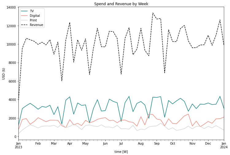
Now, we have our dependent variable. Notice how we have forced our dependent variable, revenue, to depend on our TV, digital, and print spending combined with an intercept and random noise. Figure 2 shows a weekly aggregated version of this data.

Figure 2. Weekly Aggregated Synthetic Marketing Data

Like the equation you probably learned long ago, $y = mx + b$ regressions form a line through the data. When we generated our synthetic data, we specified our $m$ as the number that multiplies our $x$ . $m$ represents our return on ad spend (ROAS) and $x$ is the spend on a channel. As you can see in Figure 3, these simple regressions approximated the original values we set.

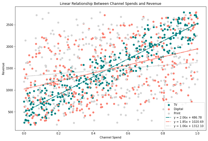
Figure 3. Fitted Lines to Individual Channel Spends and Total Revenue

Notice how the fitted lines in Figure 3 have coefficients similar to the ROASs we set on each channel. You can see this in the legend. For example, our estimated coefficient on TV spend is 2.06, whereas we set it at 2 in our synthetic dataset.

Simply regressing one channel’s spend on total revenue is not an MMM; these are all independent regressions. When we omit variables in MMMs, we can get various issues, including biasing included variables and difficulty untangling what’s influencing what (endogeneity), all of which result in misleading conclusions or predictions.

Model Development and Backtesting

As we build our model, we must analyze how good our model is at predicting what our revenue would have been. One of the primary purposes of MMMs is to make decisions about marketing budgets. As we want to decide on something in the future, our models must be able to predict the future accurately.

To measure this ability, we can run a series of tests to see how good our models are at extrapolating the future. Our accuracy should be high if our models accurately represent the world they aim to model. To test this, we split all of our historical data into two sets. One set is for training the model, and the other is for testing its accuracy on data it has yet to see. We call this backtesting. In Figure 4, you can see what this looks like in practice.

Suppose our models backtest with a high degree of accuracy. In that case, we can be confident that our models accurately represent the ecosystem we specified, and if this is the case, we can use these models to make marketing decisions.

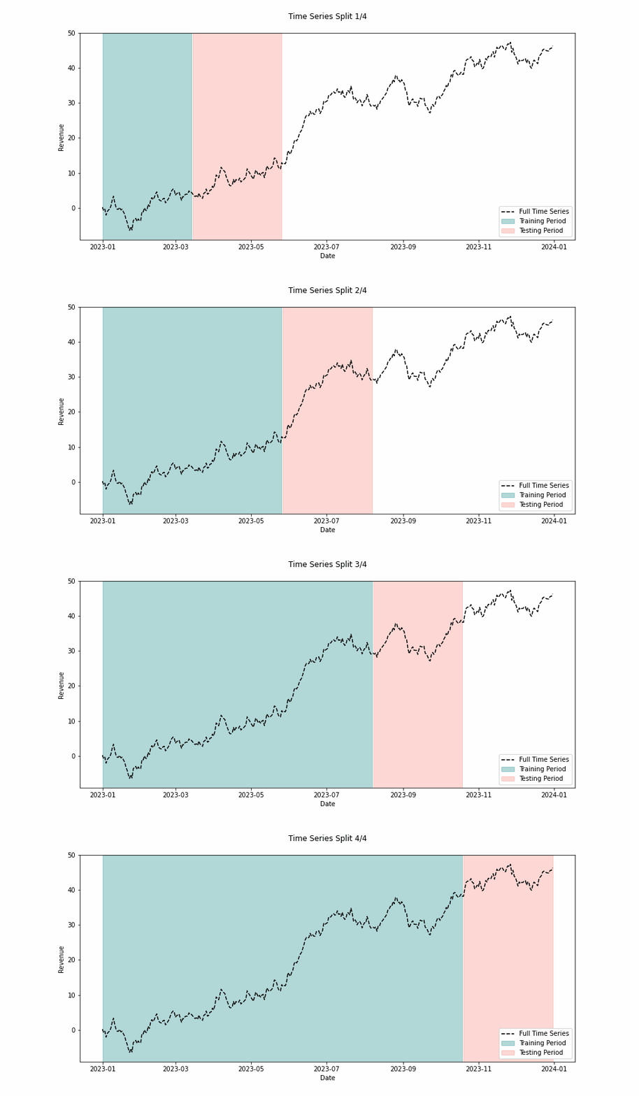
Figure 4. Visual Representation of Backtesting

Finally, to build our MMM, we must incorporate all our variables and create a multiple linear regression. Luckily for us, implementations of linear regressions are easy to come by. We must also make sure to backtest our model to validate its accuracy. Sales data is typically volatile due to seasonality, outliers, sales, and other effects. As such, repeating the backtesting process over multiple time windows is essential. We might be interested in many accuracy metrics, but one helpful metric is the root mean squared error (RMSE). A benefit of the RMSE is that it is in the same units as the dependent variable. So, it tells us the average magnitude of the errors between our predicted and observed revenue.

$\text{RMSE} = \sqrt{\frac{\sum_{i=1}^{n} (y_i - \hat{y}_i)^2}{n}}$

Here:

$n$ is the number of observations.
$y_i$ is the actual value of the dependent variable for each observation.
$\hat{y}_i$ is the predicted value of the dependent variable for each observation.

With some of the definitions out of the way, we can start to look at our model results for each time split.

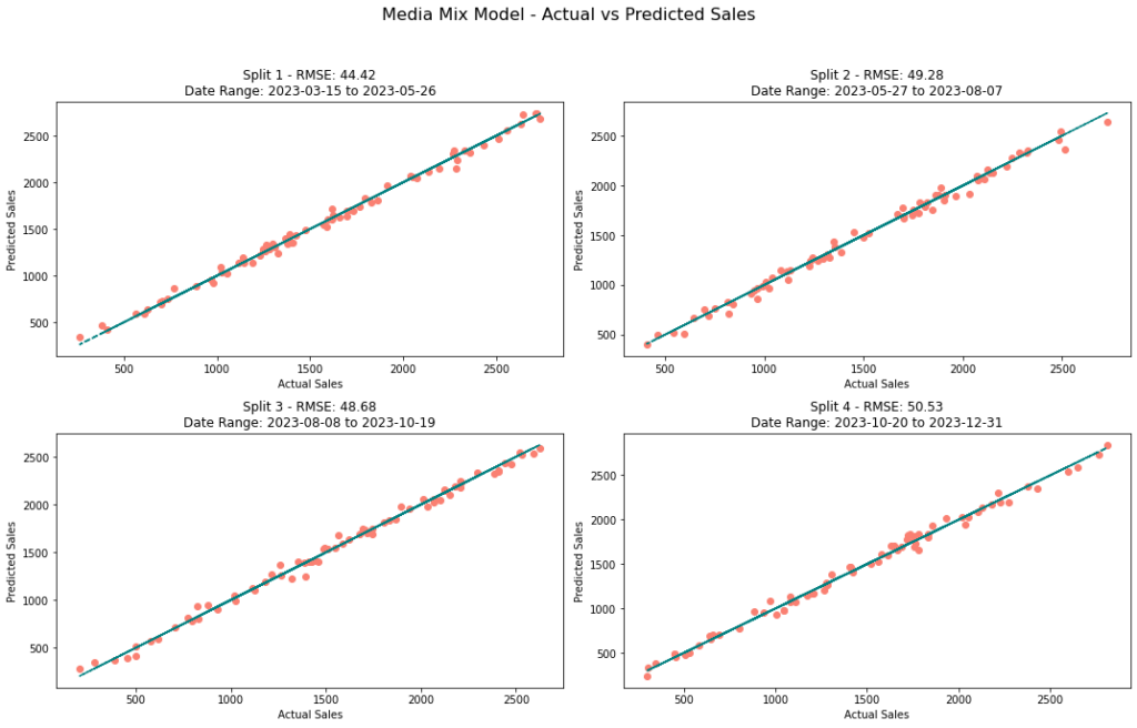
Figure 5. Backtesting Accuracies by Time Split

Figure 5 shows how our model performs in four different time frames. As you can see, the model performs well with an RMSE of about $50.00. I will include the backtesting code in my GitHub for the interested reader.

Now that we know this model performs well, we can build the complete model based on all historical data.

from sklearn.linear_model import LinearRegression

X = marketing_data[['TV', 'Digital', 'Print']]
y = marketing_data['Revenue']

model = LinearRegression()
model.fit(X, y)

With our model built, we can analyze our coefficients to validate that they match what we expect from synthetic data creation. Again, we set the coefficients (ROASs) for our channels as follows:

TV with a ROAS of 2
Digital with a ROAS of 1.5
Print with a ROAS of 1

So, our model should return with coefficients equal to those we set. If it does not, this could be due to a few factors, such as including too much noise in the synthetic data, violating the model assumptions, or overfitting.

If discrepancies exist, revisiting the data generation process, model formulation, or both may be necessary to ensure consistency and accuracy. Importantly, if the model does not perform well with our synthetic data, it likely will not perform well with our real-world data.

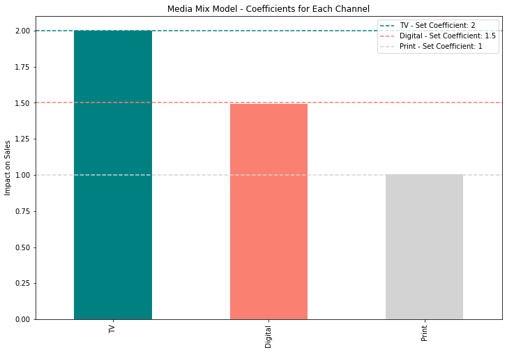
Figure 6. Bar Plot of Coefficients For Each Measured Channel

As we expected, our model recovers the parameters from our synthetic data. Because our estimated coefficients match the ROASs we set, this tells us that this model is appropriate for modeling our synthetic company data. Again, this synthetic data is all linear, so using a linear model makes the most sense, but in practice, we infrequently see pure linear relationships with marketing data.

Wrapping It Up

In conclusion, linear regression is a foundational stepping stone in media mix modeling. While real-world marketing data seldom adheres strictly to linear relationships, dismissing linear regression as “useless” oversimplifies its importance. Instead, consider it a crucial building block in your analytical toolkit. The insights from dissecting linear relationships will prove invaluable as you navigate the intricate landscape of more sophisticated modeling techniques. Understanding the basics equips you to unravel the complexity of advanced models, making linear regression an indispensable ally in the pursuit of effective media mix modeling.

Key Points:

Linear models are vital in understanding how marketing measurement functions.
Understanding the linearity assumption, model assumptions, and the shape of the data is crucial before building an MMM.
Synthetic data generation is pivotal in model validation because it provides a controlled environment to test and ensure the accuracy of known relationships.
A model that does not backtest accurately with synthetic and real-world data cannot be used for marketing measurement.

Notes:

You can find all the code for the plots here.
I have dropped the $t$ subscript in the notation to make it easier to read.